AutoGluon 时间序列 - 预测快速入门
![]()

通过简单的 fit() 调用,AutoGluon 可以训练和调优
简单的预测模型(例如,ARIMA、ETS、Theta),
强大的深度学习模型(例如,DeepAR、Temporal Fusion Transformer),
基于树的模型(例如,LightGBM),
结合其他模型预测的集成模型
为单变量时间序列数据生成多步超前*概率*预测。
本教程演示了如何快速开始使用 AutoGluon 为 M4 预测竞赛 数据集生成每小时预测。
将时间序列数据加载为 TimeSeriesDataFrame
首先,我们导入一些所需的模块
import pandas as pd
from autogluon.timeseries import TimeSeriesDataFrame, TimeSeriesPredictor
要使用 autogluon.timeseries,我们只需要以下两个类
TimeSeriesDataFrame存储包含多个时间序列的数据集。TimeSeriesPredictor负责拟合、调优和选择最佳预测模型,以及生成新的预测。
我们将 M4 每小时数据集的一个子集加载为 pandas.DataFrame
df = pd.read_csv("https://autogluon.s3.amazonaws.com/datasets/timeseries/m4_hourly_subset/train.csv")
df.head()
| item_id | timestamp | target | |
|---|---|---|---|
| 0 | H1 | 1750-01-01 00:00:00 | 605.0 |
| 1 | H1 | 1750-01-01 01:00:00 | 586.0 |
| 2 | H1 | 1750-01-01 02:00:00 | 586.0 |
| 3 | H1 | 1750-01-01 03:00:00 | 559.0 |
| 4 | H1 | 1750-01-01 04:00:00 | 511.0 |
AutoGluon 要求时间序列数据采用长格式。数据框中的每一行包含单个时间序列的一个观测值(时间步长),表示为
时间序列的唯一 ID(
"item_id"),类型为 int 或 str观测值的时间戳(
"timestamp"),类型为pandas.Timestamp或兼容格式时间序列的数值(
"target")
原始数据集应始终遵循此格式,至少包含唯一 ID、时间戳和目标值这三列,但这些列的名称可以是任意的。然而,重要的是,在构建 AutoGluon 使用的 TimeSeriesDataFrame 时,需要提供列的名称。如果数据与预期格式不符,AutoGluon 将引发异常。
train_data = TimeSeriesDataFrame.from_data_frame(
    df,
    id_column="item_id",
    timestamp_column="timestamp"
)
train_data.head()
| target | ||
|---|---|---|
| item_id | timestamp | |
| H1 | 1750-01-01 00:00:00 | 605.0 |
| 1750-01-01 01:00:00 | 586.0 | |
| 1750-01-01 02:00:00 | 586.0 | |
| 1750-01-01 03:00:00 | 559.0 | |
| 1750-01-01 04:00:00 | 511.0 |
我们将存储在 TimeSeriesDataFrame 中的每个单独时间序列称为*项目(item)*。例如,在需求预测中,项目可能对应于不同的产品;在金融数据集中,可能对应于不同的股票。这种设置也被称为时间序列*面板(panel)*。请注意,这与多元预测*不同* — AutoGluon 单独为每个时间序列生成预测,而不对不同项目(时间序列)之间的交互进行建模。
TimeSeriesDataFrame 继承自 pandas.DataFrame,因此 pandas.DataFrame 的所有属性和方法都在 TimeSeriesDataFrame 中可用。它还提供了其他实用函数,例如用于不同数据格式的加载器(详情请参阅 TimeSeriesDataFrame)。
使用 TimeSeriesPredictor.fit 训练时间序列模型
要预测时间序列的未来值,我们需要创建一个 TimeSeriesPredictor 对象。
autogluon.timeseries 中的模型对时间序列进行*多步*未来预测。我们根据任务选择这些步数 — 即*预测长度(prediction length)*(也称为*预测范围(forecast horizon)*)。例如,我们的数据集包含按小时*频率*测量的时间序列,因此我们将 prediction_length = 48 设置为训练模型,以预测未来 48 小时。
我们指示 AutoGluon 将训练好的模型保存在文件夹 ./autogluon-m4-hourly 中。我们还指定 AutoGluon 应根据平均绝对标度误差 (MASE) 对模型进行排序,并且我们想要预测的数据存储在 TimeSeriesDataFrame 的 "target" 列中。
predictor = TimeSeriesPredictor(
    prediction_length=48,
    path="autogluon-m4-hourly",
    target="target",
    eval_metric="MASE",
)

predictor.fit(
    train_data,
    presets="medium_quality",
    time_limit=600,
)
Beginning AutoGluon training... Time limit = 600s
AutoGluon will save models to '/home/ci/autogluon/docs/tutorials/timeseries/autogluon-m4-hourly'
=================== System Info ===================
AutoGluon Version:  1.3.1b20250508
Python Version:     3.11.9
Operating System:   Linux
Platform Machine:   x86_64
Platform Version:   #1 SMP Wed Mar 12 14:53:59 UTC 2025
CPU Count:          8
GPU Count:          1
Memory Avail:       28.75 GB / 30.95 GB (92.9%)
Disk Space Avail:   211.68 GB / 255.99 GB (82.7%)
===================================================
Setting presets to: medium_quality

Fitting with arguments:
{'enable_ensemble': True,
 'eval_metric': MASE,
 'hyperparameters': 'light',
 'known_covariates_names': [],
 'num_val_windows': 1,
 'prediction_length': 48,
 'quantile_levels': [0.1, 0.2, 0.3, 0.4, 0.5, 0.6, 0.7, 0.8, 0.9],
 'random_seed': 123,
 'refit_every_n_windows': 1,
 'refit_full': False,
 'skip_model_selection': False,
 'target': 'target',
 'time_limit': 600,
 'verbosity': 2}
Inferred time series frequency: 'h'
Provided train_data has 148060 rows, 200 time series. Median time series length is 700 (min=700, max=960).

Provided data contains following columns:
	target: 'target'

AutoGluon will gauge predictive performance using evaluation metric: 'MASE'
	This metric's sign has been flipped to adhere to being higher_is_better. The metric score can be multiplied by -1 to get the metric value.
===================================================

Starting training. Start time is 2025-05-08 20:52:10
Models that will be trained: ['Naive', 'SeasonalNaive', 'RecursiveTabular', 'DirectTabular', 'ETS', 'Theta', 'Chronos[bolt_small]', 'TemporalFusionTransformer']
Training timeseries model Naive. Training for up to 66.4s of the 598.0s of remaining time.
	-6.6629       = Validation score (-MASE)
	0.16    s     = Training runtime
	1.87    s     = Validation (prediction) runtime
Training timeseries model SeasonalNaive. Training for up to 74.5s of the 596.0s of remaining time.
	-1.2169       = Validation score (-MASE)
	0.15    s     = Training runtime
	0.29    s     = Validation (prediction) runtime
Training timeseries model RecursiveTabular. Training for up to 85.1s of the 595.5s of remaining time.
	-0.9339       = Validation score (-MASE)
	10.39   s     = Training runtime
	1.04    s     = Validation (prediction) runtime
Training timeseries model DirectTabular. Training for up to 97.4s of the 584.1s of remaining time.
	-1.2921       = Validation score (-MASE)
	8.23    s     = Training runtime
	0.51    s     = Validation (prediction) runtime
Training timeseries model ETS. Training for up to 115.1s of the 575.4s of remaining time.
	-1.9661       = Validation score (-MASE)
	0.14    s     = Training runtime
	24.05   s     = Validation (prediction) runtime
Training timeseries model Theta. Training for up to 137.8s of the 551.2s of remaining time.
	-2.1426       = Validation score (-MASE)
	0.14    s     = Training runtime
	1.48    s     = Validation (prediction) runtime
Training timeseries model Chronos[bolt_small]. Training for up to 183.2s of the 549.5s of remaining time.
	-0.8121       = Validation score (-MASE)
	2.10    s     = Training runtime
	1.07    s     = Validation (prediction) runtime
Training timeseries model TemporalFusionTransformer. Training for up to 273.1s of the 546.2s of remaining time.
	-2.5410       = Validation score (-MASE)
	67.38   s     = Training runtime
	0.23    s     = Validation (prediction) runtime
Fitting simple weighted ensemble.
	Ensemble weights: {'Chronos[bolt_small]': np.float64(0.74), 'DirectTabular': np.float64(0.04), 'ETS': np.float64(0.02), 'RecursiveTabular': np.float64(0.19)}
/home/ci/autogluon/timeseries/src/autogluon/timeseries/metrics/abstract.py:101: FutureWarning: Passing `prediction_length` to `TimeSeriesScorer.__call__` is deprecated and will be removed in v2.0. Please set the `eval_metric.prediction_length` attribute instead.
  warnings.warn(
	-0.7915       = Validation score (-MASE)
	0.98    s     = Training runtime
	26.67   s     = Validation (prediction) runtime
Training complete. Models trained: ['Naive', 'SeasonalNaive', 'RecursiveTabular', 'DirectTabular', 'ETS', 'Theta', 'Chronos[bolt_small]', 'TemporalFusionTransformer', 'WeightedEnsemble']
Total runtime: 120.87 s
Best model: WeightedEnsemble
Best model score: -0.7915
<autogluon.timeseries.predictor.TimeSeriesPredictor at 0x7efe043fb990>
这里我们使用了 "medium_quality" 预设,并将训练时间限制在 10 分钟(600 秒)。预设定义了 AutoGluon 将尝试拟合哪些模型。对于 medium_quality 预设,包括简单的基线模型(Naive、SeasonalNaive)、统计模型(ETS、Theta)、基于 LightGBM 的树模型(RecursiveTabular、DirectTabular)、深度学习模型 TemporalFusionTransformer,以及一个结合这些模型的加权集成。其他可用于 TimeSeriesPredictor 的预设包括 "fast_training"、"high_quality" 和 "best_quality"。更高质量的预设通常会产生更准确的预测,但训练时间更长。
在 fit() 内部,AutoGluon 将在给定的时间限制内训练尽可能多的模型。然后根据模型在内部验证集上的表现进行排名。默认情况下,此验证集是通过保留 train_data 中每个时间序列的最后 prediction_length 个时间步长来构建的。
使用 TimeSeriesPredictor.predict 生成预测
现在我们可以使用拟合好的 TimeSeriesPredictor 来预测未来的时间序列值。默认情况下,AutoGluon 将使用在内部验证集上得分最高的模型进行预测。预测总是包括从 train_data 中每个时间序列的末尾开始的未来 prediction_length 个时间步长的预测。
predictions = predictor.predict(train_data)
predictions.head()
Model not specified in predict, will default to the model with the best validation score: WeightedEnsemble
| 均值 | 0.1 | 0.2 | 0.3 | 0.4 | 0.5 | 0.6 | 0.7 | 0.8 | 0.9 | ||
|---|---|---|---|---|---|---|---|---|---|---|---|
| item_id | timestamp | ||||||||||
| H1 | 1750-01-30 04:00:00 | 622.191633 | 598.352106 | 606.819926 | 612.956287 | 617.685092 | 622.191633 | 626.836042 | 631.409826 | 636.792800 | 644.542990 |
| 1750-01-30 05:00:00 | 563.195006 | 537.393103 | 546.954576 | 553.249304 | 558.428323 | 563.195006 | 567.606607 | 572.418778 | 578.155968 | 586.702938 | |
| 1750-01-30 06:00:00 | 521.683860 | 494.428072 | 504.041315 | 511.148911 | 516.678754 | 521.683860 | 526.831450 | 532.170287 | 538.339738 | 547.689556 | |
| 1750-01-30 07:00:00 | 490.505614 | 461.721751 | 471.825645 | 479.072630 | 485.098704 | 490.505614 | 496.272718 | 502.215465 | 508.974322 | 519.732682 | |
| 1750-01-30 08:00:00 | 465.746852 | 435.351515 | 445.591065 | 453.185296 | 459.950196 | 465.746852 | 471.472651 | 477.611101 | 485.099102 | 495.941271 |
AutoGluon 生成*概率*预测:除了预测时间序列未来的均值(期望值)外,模型还提供预测分布的分位数。分位数预测让我们了解可能结果的范围。例如,如果 "0.1" 分位数等于 500.0,这意味着模型预测目标值低于 500.0 的概率为 10%。
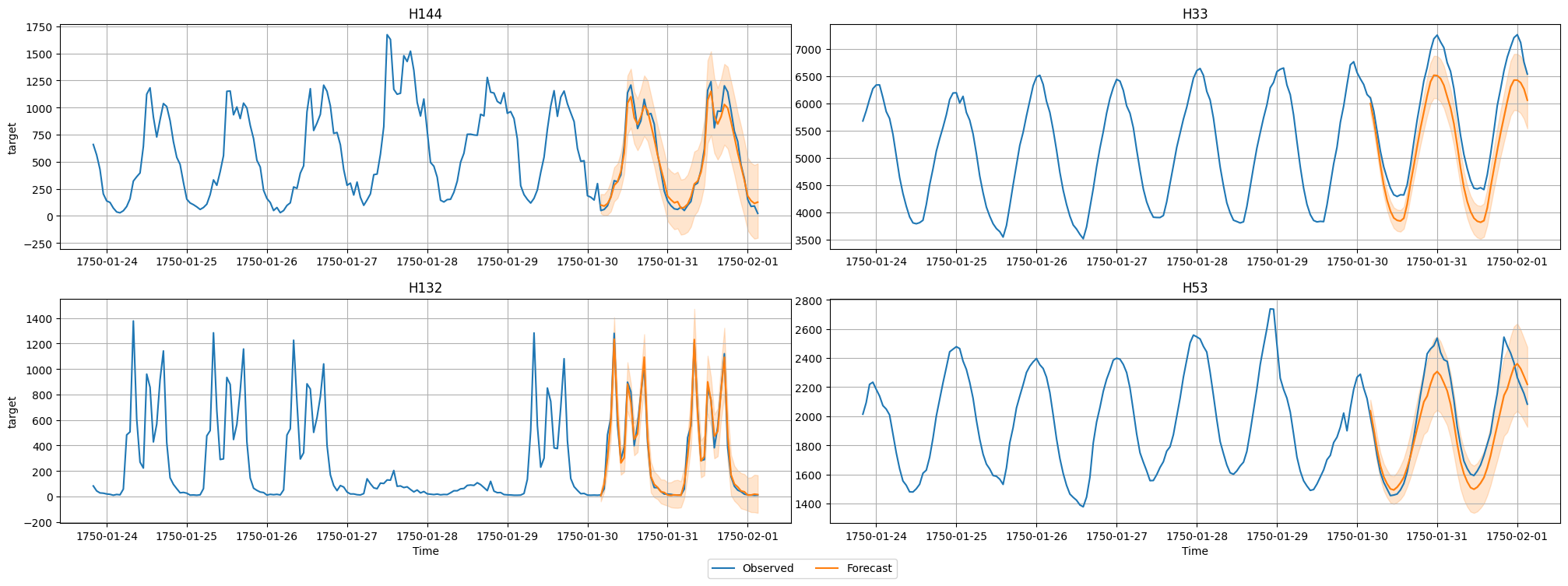
现在我们将可视化数据集中某个时间序列的预测值和实际观测值。我们绘制均值预测以及 10% 和 90% 分位数,以显示潜在结果的范围。
import matplotlib.pyplot as plt

# TimeSeriesDataFrame can also be loaded directly from a file
test_data = TimeSeriesDataFrame.from_path("https://autogluon.s3.amazonaws.com/datasets/timeseries/m4_hourly_subset/test.csv")

# Plot 4 randomly chosen time series and the respective forecasts
predictor.plot(test_data, predictions, quantile_levels=[0.1, 0.9], max_history_length=200, max_num_item_ids=4);
评估不同模型的性能
我们可以通过 leaderboard() 方法查看 AutoGluon 训练的每个模型的性能。我们将测试数据集提供给排行榜函数,以查看我们拟合的模型在未见过的测试数据上的表现。排行榜还包括在内部验证数据集上计算的验证得分。
请注意,测试数据包括预测范围(每个时间序列的最后 prediction_length 个值)以及历史数据(除最后 prediction_length 个值之外的所有值)。
在 AutoGluon 排行榜中,更高的得分始终对应于更好的预测性能。因此,我们的 MASE 分数乘以 -1,以便更高的“负 MASE”对应于更准确的预测。
# The test score is computed using the last
# prediction_length=48 timesteps of each time series in test_data
predictor.leaderboard(test_data)
Additional data provided, testing on additional data. Resulting leaderboard will be sorted according to test score (`score_test`).
/home/ci/autogluon/timeseries/src/autogluon/timeseries/metrics/abstract.py:101: FutureWarning: Passing `prediction_length` to `TimeSeriesScorer.__call__` is deprecated and will be removed in v2.0. Please set the `eval_metric.prediction_length` attribute instead.
  warnings.warn(
/home/ci/autogluon/timeseries/src/autogluon/timeseries/metrics/abstract.py:101: FutureWarning: Passing `prediction_length` to `TimeSeriesScorer.__call__` is deprecated and will be removed in v2.0. Please set the `eval_metric.prediction_length` attribute instead.
  warnings.warn(
/home/ci/autogluon/timeseries/src/autogluon/timeseries/metrics/abstract.py:101: FutureWarning: Passing `prediction_length` to `TimeSeriesScorer.__call__` is deprecated and will be removed in v2.0. Please set the `eval_metric.prediction_length` attribute instead.
  warnings.warn(
/home/ci/autogluon/timeseries/src/autogluon/timeseries/metrics/abstract.py:101: FutureWarning: Passing `prediction_length` to `TimeSeriesScorer.__call__` is deprecated and will be removed in v2.0. Please set the `eval_metric.prediction_length` attribute instead.
  warnings.warn(
/home/ci/autogluon/timeseries/src/autogluon/timeseries/metrics/abstract.py:101: FutureWarning: Passing `prediction_length` to `TimeSeriesScorer.__call__` is deprecated and will be removed in v2.0. Please set the `eval_metric.prediction_length` attribute instead.
  warnings.warn(
/home/ci/autogluon/timeseries/src/autogluon/timeseries/metrics/abstract.py:101: FutureWarning: Passing `prediction_length` to `TimeSeriesScorer.__call__` is deprecated and will be removed in v2.0. Please set the `eval_metric.prediction_length` attribute instead.
  warnings.warn(
/home/ci/autogluon/timeseries/src/autogluon/timeseries/metrics/abstract.py:101: FutureWarning: Passing `prediction_length` to `TimeSeriesScorer.__call__` is deprecated and will be removed in v2.0. Please set the `eval_metric.prediction_length` attribute instead.
  warnings.warn(
/home/ci/autogluon/timeseries/src/autogluon/timeseries/metrics/abstract.py:101: FutureWarning: Passing `prediction_length` to `TimeSeriesScorer.__call__` is deprecated and will be removed in v2.0. Please set the `eval_metric.prediction_length` attribute instead.
  warnings.warn(
/home/ci/autogluon/timeseries/src/autogluon/timeseries/metrics/abstract.py:101: FutureWarning: Passing `prediction_length` to `TimeSeriesScorer.__call__` is deprecated and will be removed in v2.0. Please set the `eval_metric.prediction_length` attribute instead.
  warnings.warn(
| 模型 | 测试得分 | 验证得分 | 测试预测时间 | 验证预测时间 | 边际拟合时间 | 拟合顺序 | |
|---|---|---|---|---|---|---|---|
| 0 | WeightedEnsemble | -0.697903 | -0.791454 | 31.927198 | 26.674226 | 0.976847 | 9 |
| 1 | Chronos[bolt_small] | -0.725739 | -0.812070 | 0.785397 | 1.070726 | 2.103007 | 7 |
| 2 | RecursiveTabular | -0.862797 | -0.933874 | 1.047061 | 1.038171 | 10.387928 | 3 |
| 3 | SeasonalNaive | -1.022854 | -1.216909 | 0.167951 | 0.291220 | 0.148167 | 2 |
| 4 | DirectTabular | -1.605700 | -1.292127 | 0.555017 | 0.510770 | 8.234862 | 4 |
| 5 | ETS | -1.806136 | -1.966098 | 29.531827 | 24.054558 | 0.144623 | 5 |
| 6 | Theta | -1.905367 | -2.142551 | 1.672346 | 1.481339 | 0.141250 | 6 |
| 7 | TemporalFusionTransformer | -2.272206 | -2.540983 | 0.308293 | 0.226115 | 67.381492 | 8 |
| 8 | Naive | -6.696079 | -6.662942 | 0.172883 | 1.872083 | 0.156657 | 1 |
总结
我们使用 autogluon.timeseries 对 M4 每小时数据集进行了概率多步预测。请查看 时间序列预测 - 深入,了解 AutoGluon 在时间序列预测方面的更高级功能。