时间序列预测 - 深度解析

本教程深入概述了 AutoGluon 中的时间序列预测功能。具体来说，我们将涵盖：

• 什么是概率时间序列预测？

• 使用额外信息进行时间序列预测

• TimeSeriesPredictor 期望的数据格式是什么？

• 如何评估预测准确性？

• AutoGluon 中有哪些可用的预测模型？

• TimeSeriesPredictor 提供哪些功能？

  • 使用 presets 和 time_limit 进行基本配置

  • 手动选择要训练的模型

  • 超参数调优

本教程假定您熟悉时间序列预测 - 快速入门中的内容。

什么是概率时间序列预测？

时间序列是按固定间隔进行的测量序列。时间序列预测的主要目标是根据过去观测值预测时间序列的未来值。这项任务的一个典型示例是需求预测。例如，我们可以将某种产品的每日购买数量表示为时间序列。在这种情况下，目标可能是根据历史购买数据预测未来 14 天（即预测期）中每一天的需求。在 AutoGluon 中，TimeSeriesPredictor 的 prediction_length 参数决定了预测期的长度。

预测的目标可以是预测给定时间序列的未来值，以及建立未来值可能落入的预测区间。在 AutoGluon 中，TimeSeriesPredictor 生成两种类型的预测：

• 均值预测 表示预测期内每个时间步长的时间序列预期值。

• 分位数预测 表示预测分布的分位数。例如，如果 0.1 分位数（也称为 P10 或第 10 个百分位数）等于 x，则意味着时间序列值有 10% 的时间预计会低于 x。再举一个例子，0.5 分位数（P50）对应于中位数预测。分位数可用于推断可能结果的范围。例如，根据分位数的定义，时间序列值有 80% 的概率会介于 P10 和 P90 之间。

默认情况下，TimeSeriesPredictor 输出分位数 [0.1, 0.2, 0.3, 0.4, 0.5, 0.6, 0.7, 0.8, 0.9]。可以使用 quantile_levels 参数提供自定义分位数：

predictor = TimeSeriesPredictor(quantile_levels=[0.05, 0.5, 0.95])

使用额外信息进行时间序列预测

在实际的时间序列预测问题中，除了原始时间序列值之外，我们通常还可以获得额外信息。AutoGluon 支持两种此类额外信息：静态特征和时变协变量。

注意

并非 AutoGluon 中所有模型都支持所有类型的特征 & 协变量。有关概述，请参见预测模型库 / 额外特征。

静态特征

静态特征是时间序列的时间无关属性（元数据）。这些信息可能包括：

• 记录时间序列的位置（国家、州、城市）

• 产品的固定属性（品牌名称、颜色、尺寸、重量）

• 商店 ID 或产品 ID

例如，提供这些信息有助于预测模型为位于同一城市的商店生成相似的需求预测。

在 AutoGluon 中，静态特征存储为 TimeSeriesDataFrame 对象的一个属性。例如，我们来看一下 M4 Daily 数据集。

import pandas as pd
from autogluon.timeseries import TimeSeriesDataFrame, TimeSeriesPredictor

我们从 M4 Daily 数据集中下载 100 个时间序列的子集。

df = pd.read_csv("https://autogluon.s3.amazonaws.com/datasets/timeseries/m4_daily_subset/train.csv")
df.head()

	item_id	timestamp	target
0	D1737	1995-05-23	1900.0
1	D1737	1995-05-24	1877.0
2	D1737	1995-05-25	1873.0
3	D1737	1995-05-26	1859.0
4	D1737	1995-05-27	1876.0

我们还加载了相应的静态特征。在 M4 Daily 数据集中，有一个单一的类别静态特征，表示每个时间序列的来源领域。

static_features_df = pd.read_csv("https://autogluon.s3.amazonaws.com/datasets/timeseries/m4_daily_subset/metadata.csv")
static_features_df.head()

	item_id	domain
0	D1737	Industry
1	D1843	Industry
2	D2246	Finance
3	D909	Micro
4	D1345	Micro

AutoGluon 期望静态特征是 pandas.DataFrame 对象。item_id 列指示了 static_features 的每一行对应于 df 中哪个 item（=单个时间序列）。

现在我们可以创建一个 TimeSeriesDataFrame，其中包含时间序列值和静态特征。

train_data = TimeSeriesDataFrame.from_data_frame(
    df,
    id_column="item_id",
    timestamp_column="timestamp",
    static_features_df=static_features_df,
)
train_data.head()

		target
item_id	timestamp
D1737	1995-05-23	1900.0
	1995-05-24	1877.0
	1995-05-25	1873.0
	1995-05-26	1859.0
	1995-05-27	1876.0

我们可以使用 .static_features 属性验证 train_data 现在也包含静态特征：

train_data.static_features.head()

	domain
item_id
D1737	Industry
D1843	Industry
D2246	Finance
D909	Micro
D1345	Micro

或者，我们可以通过分配 .static_features 属性将静态特征附加到现有的 TimeSeriesDataFrame 上：

train_data.static_features = static_features_df

如果 static_features 不包含 train_data 中存在的一些 item_id，将会引发异常。

现在，当我们拟合预测器时，所有支持静态特征的模型将自动使用 train_data 中包含的静态特征。

predictor = TimeSeriesPredictor(prediction_length=14).fit(train_data)

...
Following types of static features have been inferred:
	categorical: ['domain']
	continuous (float): []
...

此消息确认列 'domain' 被解释为类别特征。通常，AutoGluon-TimeSeries 支持两种类型的静态特征：

• categorical：dtype 为 object, string 和 category 的列被解释为离散类别

• continuous：dtype 为 int 和 float 的列被解释为连续（实数值）数字

• 其他 dtypes 的列将被忽略

要覆盖此逻辑，我们需要手动更改列的 dtype。例如，假设静态特征数据框包含一个整数值列 "store_id"。

train_data.static_features["store_id"] = list(range(len(train_data.item_ids)))

默认情况下，此列将被解释为连续数字。我们可以通过将 dtype 更改为 category 来强制 AutoGluon 将其解释为类别特征。

train_data.static_features["store_id"] = train_data.static_features["store_id"].astype("category")

注意：如果训练数据包含静态特征，预测器会要求传递给 predictor.predict()、predictor.leaderboard() 和 predictor.evaluate() 的数据也包含具有相同列名和数据类型的静态特征。

时变协变量

协变量是可能影响目标时间序列的时变特征。有时它们也被称为动态特征、外生回归量或相关时间序列。AutoGluon 支持两种类型的协变量：

• 已知协变量，在整个预测期内已知，例如：

  • 节假日

  • 星期几、月份、年份

  • 促销活动

• 过去协变量，仅在预测期开始时已知，例如：

  • 其他产品的销售额

  • 温度、降水量

  • 转换后的目标时间序列

在 AutoGluon 中，known_covariates 和 past_covariates 都作为附加列存储在 TimeSeriesDataFrame 中。

我们将再次使用 M4 Daily 数据集作为示例，生成这两种类型的协变量：

• 一个 past_covariate，等于目标时间序列的对数

• 一个 known_covariate，如果给定日期是周末则等于 1，否则等于 0。

import numpy as np
train_data["log_target"] = np.log(train_data["target"])

WEEKEND_INDICES = [5, 6]
timestamps = train_data.index.get_level_values("timestamp")
train_data["weekend"] = timestamps.weekday.isin(WEEKEND_INDICES).astype(float)

train_data.head()

		target	log_target	weekend
item_id	timestamp
D1737	1995-05-23	1900.0	7.549609	0.0
	1995-05-24	1877.0	7.537430	0.0
	1995-05-25	1873.0	7.535297	0.0
	1995-05-26	1859.0	7.527794	0.0
	1995-05-27	1876.0	7.536897	1.0

创建 TimeSeriesPredictor 时，我们指定列 "target" 是我们的预测目标，列 "weekend" 包含在预测时已知的协变量。

predictor = TimeSeriesPredictor(
    prediction_length=14,
    target="target",
    known_covariates_names=["weekend"],
).fit(train_data)

预测器会自动将剩余列（目标和已知协变量除外）解释为过去协变量。此信息在拟合期间会被记录下来：

...
Provided dataset contains following columns:
	target:           'target'
	known covariates: ['weekend']
	past covariates:  ['log_target']
...

最后，为了进行预测，我们为预测期生成已知协变量：

predictor = TimeSeriesPredictor(prediction_length=14, freq=train_data.freq)

known_covariates = predictor.make_future_data_frame(train_data)
known_covariates["weekend"] = known_covariates["timestamp"].dt.weekday.isin(WEEKEND_INDICES).astype(float)

known_covariates.head()

	item_id	timestamp	weekend
0	D1069	2013-01-20	1.0
1	D1069	2013-01-21	0.0
2	D1069	2013-01-22	0.0
3	D1069	2013-01-23	0.0
4	D1069	2013-01-24	0.0

请注意，known_covariates 必须满足以下条件：

• 列必须包含 predictor.known_covariates_names 中列出的所有列

• item_id 索引必须包含 train_data 中存在的所有 item id

• timestamp 索引必须包含 train_data 中每个时间序列末尾 prediction_length 个未来时间步的值

如果 known_covariates 包含比必要信息更多（例如，包含额外的列、item_id 或 timestamp），AutoGluon 将自动选择必要的行和列。

最后，我们将 known_covariates 传递给 predict 函数以生成预测：

predictor.predict(train_data, known_covariates=known_covariates)

支持静态特征和协变量的模型列表可在预测模型库中找到。

节假日

known_covariates 的另一个常见示例是节假日特征。本节介绍如何将节假日特征添加到时间序列数据集中并在 AutoGluon 中使用它们。

首先，我们需要定义一个字典，其键为 datetime.date 格式的日期，值为节假日名称。我们可以轻松使用 holidays Python 包生成这样的字典。

!pip install -q holidays

这里我们仅使用德国节假日进行演示。请务必定义一个与您国家/地区匹配的节假日日历！

import holidays

timestamps = train_data.index.get_level_values("timestamp")
country_holidays = holidays.country_holidays(
    country="DE",  # make sure to select the correct country/region!
    # Add + 1 year to make sure that holidays are initialized for the forecast horizon
    years=range(timestamps.min().year, timestamps.max().year + 1),
)
# Convert dict to pd.Series for pretty visualization
pd.Series(country_holidays).sort_index().head()

1990-10-03             German Unity Day
1990-11-21    Repentance and Prayer Day
1990-12-25                Christmas Day
1990-12-26      Second Day of Christmas
1991-01-01               New Year's Day
dtype: object

或者，我们可以手动定义一个包含自定义节假日的字典。

import datetime

# must cover the full train time range + forecast horizon
custom_holidays = {
    datetime.date(1995, 1, 29): "Superbowl",
    datetime.date(1995, 11, 29): "Black Friday",
    datetime.date(1996, 1, 28): "Superbowl",
    datetime.date(1996, 11, 29): "Black Friday",
    # ...
}

接下来，我们定义一个方法，将节假日特征作为列添加到 TimeSeriesDataFrame 中。

def add_holiday_features(
    ts_df: TimeSeriesDataFrame,
    country_holidays: dict,
    include_individual_holidays: bool = True,
    include_holiday_indicator: bool = True,
) -> TimeSeriesDataFrame:
    """Add holiday indicator columns to a TimeSeriesDataFrame."""
    ts_df = ts_df.copy()
    if not isinstance(ts_df, TimeSeriesDataFrame):
        ts_df = TimeSeriesDataFrame(ts_df)
    timestamps = ts_df.index.get_level_values("timestamp")
    country_holidays_df = pd.get_dummies(pd.Series(country_holidays)).astype(float)
    holidays_df = country_holidays_df.reindex(timestamps.date).fillna(0)
    if include_individual_holidays:
        ts_df[holidays_df.columns] = holidays_df.values
    if include_holiday_indicator:
        ts_df["Holiday"] = holidays_df.max(axis=1).values
    return ts_df

我们可以为所有节假日创建一个单一的指示器特征。

add_holiday_features(train_data, country_holidays, include_individual_holidays=False).head()

		target	log_target	weekend	Holiday
item_id	timestamp
D1737	1995-05-23	1900.0	7.549609	0.0	0.0
	1995-05-24	1877.0	7.537430	0.0	0.0
	1995-05-25	1873.0	7.535297	0.0	1.0
	1995-05-26	1859.0	7.527794	0.0	0.0
	1995-05-27	1876.0	7.536897	1.0	0.0

或者用单独的特征表示每个节假日。

train_data_with_holidays = add_holiday_features(train_data, country_holidays)
train_data_with_holidays.head()

		target	log_target	weekend	Ascension Day	Ascension Day; Labor Day	Christmas Day	Easter Monday	German Unity Day	Good Friday	Labor Day	New Year's Day	Reformation Day	Repentance and Prayer Day	Second Day of Christmas	Whit Monday	Holiday
item_id	timestamp
D1737	1995-05-23	1900.0	7.549609	0.0	0.0	0.0	0.0	0.0	0.0	0.0	0.0	0.0	0.0	0.0	0.0	0.0	0.0
	1995-05-24	1877.0	7.537430	0.0	0.0	0.0	0.0	0.0	0.0	0.0	0.0	0.0	0.0	0.0	0.0	0.0	0.0
	1995-05-25	1873.0	7.535297	0.0	1.0	0.0	0.0	0.0	0.0	0.0	0.0	0.0	0.0	0.0	0.0	0.0	1.0
	1995-05-26	1859.0	7.527794	0.0	0.0	0.0	0.0	0.0	0.0	0.0	0.0	0.0	0.0	0.0	0.0	0.0	0.0
	1995-05-27	1876.0	7.536897	1.0	0.0	0.0	0.0	0.0	0.0	0.0	0.0	0.0	0.0	0.0	0.0	0.0	0.0

请记住在创建 TimeSeriesPredictor 时将节假日特征名称添加为 known_covariates_names。

holiday_columns = train_data_with_holidays.columns.difference(train_data.columns)
predictor = TimeSeriesPredictor(..., known_covariates_names=holiday_columns).fit(train_data_with_holidays, ...)

在预测时，我们需要将未来的节假日值作为 known_covariates 提供。

known_covariates = predictor.make_future_data_frame(train_data)
known_covariates = add_holiday_features(known_covariates, country_holidays)
known_covariates.head()

		Ascension Day	Ascension Day; Labor Day	Christmas Day	Easter Monday	German Unity Day	Good Friday	Labor Day	New Year's Day	Reformation Day	Repentance and Prayer Day	Second Day of Christmas	Whit Monday	Holiday
item_id	timestamp
D1069	2013-01-20	0.0	0.0	0.0	0.0	0.0	0.0	0.0	0.0	0.0	0.0	0.0	0.0	0.0
	2013-01-21	0.0	0.0	0.0	0.0	0.0	0.0	0.0	0.0	0.0	0.0	0.0	0.0	0.0
	2013-01-22	0.0	0.0	0.0	0.0	0.0	0.0	0.0	0.0	0.0	0.0	0.0	0.0	0.0
	2013-01-23	0.0	0.0	0.0	0.0	0.0	0.0	0.0	0.0	0.0	0.0	0.0	0.0	0.0
	2013-01-24	0.0	0.0	0.0	0.0	0.0	0.0	0.0	0.0	0.0	0.0	0.0	0.0	0.0

predictions = predictor.predict(train_data_with_holidays, known_covariates=known_covariates)

TimeSeriesPredictor 期望的数据格式是什么？

AutoGluon 要求训练数据中至少有一些时间序列足够长，以便生成内部验证集。

这意味着，在使用默认设置进行训练时，train_data 中至少有一些时间序列的长度必须 >= max(prediction_length + 1, 5) + prediction_length

predictor = TimeSeriesPredictor(prediction_length=prediction_length).fit(train_data)

如果您使用高级配置选项，例如以下内容，

predictor = TimeSeriesPredictor(prediction_length=prediction_length).fit(train_data, num_val_windows=num_val_windows, val_step_size=val_step_size)

则 train_data 中至少有一些时间序列的长度必须 >= max(prediction_length + 1, 5) + prediction_length + (num_val_windows - 1) * val_step_size。

请注意，数据集中所有时间序列的长度可以不同。

处理不规则数据和缺失值

在某些应用中，例如金融领域，数据通常带有不规则的测量值（例如，周末或节假日没有股票价格）或缺失值。

这是一个带有不规则时间索引的数据集示例：

df_irregular = TimeSeriesDataFrame(
    pd.DataFrame(
        {
            "item_id": [0, 0, 0, 1, 1],
            "timestamp": ["2022-01-01", "2022-01-02", "2022-01-04", "2022-01-01", "2022-01-04"],
            "target": [1, 2, 3, 4, 5],
        }
    )
)
df_irregular

		target
item_id	timestamp
0	2022-01-01	1
	2022-01-02	2
	2022-01-04	3
1	2022-01-01	4
	2022-01-04	5

在这种情况下，您可以在创建预测器时使用 freq 参数指定所需的频率。

predictor = TimeSeriesPredictor(..., freq="D").fit(df_irregular)

这里我们选择 freq="D" 表示填充后的索引必须具有每日频率（参见pandas 文档中的其他可能选择）。

AutoGluon 将自动把不规则数据转换为每日频率并处理缺失值。

---

或者，我们可以使用方法 TimeSeriesDataFrame.convert_frequency() 手动填充时间索引中的空白。

df_regular = df_irregular.convert_frequency(freq="D")
df_regular

		target
item_id	timestamp
0	2022-01-01	1.0
	2022-01-02	2.0
	2022-01-03	NaN
	2022-01-04	3.0
1	2022-01-01	4.0
	2022-01-02	NaN
	2022-01-03	NaN
	2022-01-04	5.0

我们可以验证索引现在是规则的，并且具有每日频率：

print(f"Data has frequency '{df_regular.freq}'")

Data has frequency 'D'

现在数据包含由 NaN 表示的缺失值。AutoGluon 中的大多数时间序列模型可以原生处理缺失值，因此我们可以直接将数据传递给 TimeSeriesPredictor。

或者，我们可以使用 TimeSeriesDataFrame.fill_missing_values() 方法通过适当的策略手动填充 NaN。默认情况下，缺失值使用前向填充 + 后向填充的组合进行填充。

df_filled = df_regular.fill_missing_values()
df_filled

		target
item_id	timestamp
0	2022-01-01	1.0
	2022-01-02	2.0
	2022-01-03	2.0
	2022-01-04	3.0
1	2022-01-01	4.0
	2022-01-02	4.0
	2022-01-03	4.0
	2022-01-04	5.0

在某些应用中，例如需求预测，缺失值可能对应于零需求。在这种情况下，常数填充更合适。

df_filled = df_regular.fill_missing_values(method="constant", value=0.0)
df_filled

		target
item_id	timestamp
0	2022-01-01	1.0
	2022-01-02	2.0
	2022-01-03	0.0
	2022-01-04	3.0
1	2022-01-01	4.0
	2022-01-02	0.0
	2022-01-03	0.0
	2022-01-04	5.0

如何评估预测准确性？

为了衡量 TimeSeriesPredictor 预测未知时间序列的准确性，我们需要保留一些不用于训练的测试数据。这可以通过使用 TimeSeriesDataFrame 的 train_test_split 方法轻松完成：

prediction_length = 48
data = TimeSeriesDataFrame.from_path("https://autogluon.s3.amazonaws.com/datasets/timeseries/m4_hourly_subset/train.csv")
train_data, test_data = data.train_test_split(prediction_length)

Sorting the dataframe index before generating the train/test split.

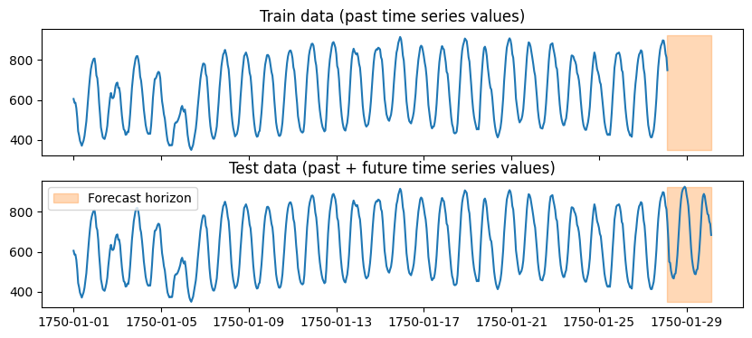
我们从原始数据中获得了两个 TimeSeriesDataFrame

• test_data 包含与原始 data 完全相同的数据（即，它包含历史数据和预测期）

• 在 train_data 中，从每个时间序列的末尾移除最后的 prediction_length 个时间步（即，它仅包含历史数据）

import matplotlib.pyplot as plt
import numpy as np

item_id = "H1"
fig, (ax1, ax2) = plt.subplots(nrows=2, figsize=[10, 4], sharex=True)
train_ts = train_data.loc[item_id]
test_ts = test_data.loc[item_id]
ax1.set_title("Train data (past time series values)")
ax1.plot(train_ts)
ax2.set_title("Test data (past + future time series values)")
ax2.plot(test_ts)
for ax in (ax1, ax2):
    ax.fill_between(np.array([train_ts.index[-1], test_ts.index[-1]]), test_ts.min(), test_ts.max(), color="C1", alpha=0.3, label="Forecast horizon")
plt.legend()
plt.show()

现在我们可以使用 train_data 训练预测器，并使用 test_data 获得其在未知数据上性能的估计。

predictor = TimeSeriesPredictor(prediction_length=prediction_length, eval_metric="MASE").fit(train_data)
predictor.evaluate(test_data)

AutoGluon 通过衡量预测模型的预测与实际观测时间序列的匹配程度来评估其性能。对于 test_data 中的每个时间序列，预测器执行以下操作：

1. 保留时间序列最后的 prediction_length 个值。

2. 为时间序列的保留部分（即预测期）生成预测。

3. 使用 eval_metric 量化预测与时间序列实际观测（保留）值的匹配程度。

最后，将分数在数据集中的所有时间序列上取平均。

这里的关键细节是 evaluate 总是计算每个时间序列最后 prediction_length 个时间步上的分数。每个时间序列的开始部分（除了最后 prediction_length 个时间步）仅用于在预测之前初始化模型。

有关评估指标的更多详细信息，请参见预测评估指标。

使用多个截止点进行回测

我们可以使用回测（即，评估从同一时间序列生成的多个预测期上的性能）更准确地估计性能。

这可以通过将 cutoff 参数传递给 evaluate 方法来完成。

num_val_windows = 3
for cutoff in range(-num_val_windows * prediction_length, 0, step=prediction_length):
    score = predictor.evaluate(test_data, cutoff=cutoff)
    print(f"Cutoff {cutoff}: score = {score}")

evaluate 方法将使用截止点索引之后的 prediction_length 个时间步作为保留集（标记为橙色）来衡量预测准确性。默认情况下（如果未提供 cutoff），cutoff 值将设置为 -1 * prediction_length。

如果您想一次评估多个模型，您可以类似地将不同的 cutoff 值提供给 leaderboard 方法。

多窗口回测通常能更准确地估计未知数据上的预测质量。然而，这种策略会减少可用于拟合模型的训练数据量，因此如果训练时间序列较短，我们建议使用单窗口回测。

AutoGluon 如何执行验证？

当我们使用 predictor.fit(train_data=train_data) 拟合预测器时，AutoGluon 在底层会将原始数据集 train_data 进一步分割成训练集和验证集。

使用 evaluate 方法评估不同模型在验证集上的性能，就像上面描述的那样。最终将使用在验证集上获得最佳分数的模型进行预测。

默认情况下，内部验证集包含一个单窗口，其中包含每个时间序列最后 prediction_length 个时间步。我们可以使用 num_val_windows 参数增加验证窗口的数量。

predictor = TimeSeriesPredictor(...)
predictor.fit(train_data, num_val_windows=3)

这将减少过拟合的可能性，但会使训练时间大致增加 num_val_windows 倍。请注意，只有当 train_data 中的时间序列长度至少为 (num_val_windows + 1) * prediction_length 时，才能使用多个验证窗口。

或者，用户可以向 fit 方法提供自己的验证集。在这种情况下，重要的是要记住验证分数是在每个时间序列最后的 prediction_length 个时间步上计算的。

predictor.fit(train_data=train_data, tuning_data=my_validation_dataset)

AutoGluon 中有哪些可用的预测模型？

AutoGluon 中的预测模型可以分为三大类：局部模型、全局模型和集成模型。

局部模型 是简单的统计模型，专门设计用于捕捉趋势或季节性等模式。尽管简单，这些模型通常能产生合理的预测，并作为强大的基准。一些可用的局部模型示例：

• ETS

• AutoARIMA

• Theta

• SeasonalNaive

如果数据集包含多个时间序列，我们会为每个时间序列拟合一个单独的局部模型——因此得名“局部”。这意味着，如果我们想为不属于训练集的新时间序列进行预测，所有局部模型都将从头开始为新时间序列进行拟合。

全局模型 是机器学习算法，它们从包含多个时间序列的整个训练集中学习一个单一模型。AutoGluon 中的大多数全局模型由 GluonTS 库提供。这些是用 PyTorch 实现的神经网络算法，例如：

• DeepAR

• PatchTST

• DLinear

• TemporalFusionTransformer

此类模型还包括像Chronos这样的预训练零样本预测模型。

AutoGluon 还提供了两个表格全局模型 RecursiveTabular 和 DirectTabular。在底层，这些模型将预测任务转换为回归问题，并使用 TabularPredictor 来拟合 LightGBM 等回归算法。

最后，集成模型 通过组合所有其他模型的预测进行工作。默认情况下，TimeSeriesPredictor 总是拟合一个 WeightedEnsemble 在其他模型之上。在调用 fit 方法时通过设置 enable_ensemble=False 可以禁用此功能。

有关每个模型可调超参数的列表、其默认值和其他详细信息，请参见预测模型库。

TimeSeriesPredictor 提供哪些功能？

AutoGluon 提供了多种配置 TimeSeriesPredictor 行为的方式，适合初学者和专家用户。

使用 presets 和 time_limit 进行基本配置

我们可以使用 fit 方法的 presets 参数，以不同的预定义配置拟合 TimeSeriesPredictor。

predictor = TimeSeriesPredictor(...)
predictor.fit(train_data, presets="medium_quality")

更高质量的预设通常会产生更好的预测，但训练时间更长。以下预设可用：

预设	描述	用例	拟合时间（理想）
fast_training	拟合简单统计模型和基准模型 + 快速树模型	训练快但准确性可能不高	0.5x
medium_quality	与 fast_training 中的模型相同 + 深度学习模型 TemporalFusionTransformer + Chronos-Bolt（小）	预测效果好，训练时间合理	1x
high_quality	更强大的深度学习、机器学习、统计和预训练预测模型	比 medium_quality 准确性高得多，但训练时间更长	3x
best_quality	与 high_quality 中的模型相同，更多交叉验证窗口	通常比 high_quality 更准确，特别是对于时间序列较少（<50 个）的数据集	6x

您可以在 AutoGluon 源代码中找到有关预设和每个预设中包含的模型的更多信息。

控制训练时间的另一种方法是使用 time_limit 参数。

predictor.fit(
    train_data,
    time_limit=60 * 60,  # total training time in seconds
)

如果未提供 time_limit，预测器将一直训练直到所有模型拟合完成。

手动配置模型

高级用户可以覆盖预设，并使用 hyperparameters 参数手动指定预测器应训练哪些模型。

predictor = TimeSeriesPredictor(...)

predictor.fit(
    ...
    hyperparameters={
        "DeepAR": {},
        "Theta": [
            {"decomposition_type": "additive"},
            {"seasonal_period": 1},
        ],
    }
)

上面的示例将训练三个模型：

• 使用默认超参数的 DeepAR

• 使用加性季节性分解的 Theta（所有其他参数设置为默认值）

• 禁用季节性的 Theta（所有其他参数设置为默认值）

您还可以使用 excluded_model_type 参数从预设中排除某些模型。

predictor.fit(
    ...
    presets="high_quality",
    excluded_model_types=["AutoETS", "AutoARIMA"],
)

有关可用模型及其相应超参数的完整列表，请参见预测模型库。

超参数调优

高级用户可以为模型超参数定义搜索空间，让 AutoGluon 自动确定模型的最佳配置。

from autogluon.common import space

predictor = TimeSeriesPredictor()

predictor.fit(
    train_data,
    hyperparameters={
        "DeepAR": {
            "hidden_size": space.Int(20, 100),
            "dropout_rate": space.Categorical(0.1, 0.3),
        },
    },
    hyperparameter_tune_kwargs="auto",
    enable_ensemble=False,
)

此代码将训练 DeepAR 模型的多个版本，采用 10 种不同的超参数配置。AutoGluon 将自动选择在验证集上获得最高分数的最佳模型配置并用于预测。

目前，深度学习模型（来自 GluonTS）的 HPO 基于 Ray Tune，所有其他时间序列模型则使用随机搜索。

我们可以通过将字典作为 hyperparameter_tune_kwargs 传递来更改每个模型的随机搜索试验次数。

predictor.fit(
    ...
    hyperparameter_tune_kwargs={
        "num_trials": 20,
        "scheduler": "local",
        "searcher": "random",
    },
    ...
)

hyperparameter_tune_kwargs 字典必须包含以下键：

• "num_trials": int，每个调优模型的训练配置数量

• "searcher": 目前唯一支持的选项是 "random" (随机搜索)。

• "scheduler": 目前唯一支持的选项是 "local" (所有模型在同一机器上训练)

注意：HPO 会显著增加大多数模型的训练时间，但通常只能带来适度的性能提升。