使用 AutoMM 进行文本语义搜索¶

1. 语义嵌入简介¶

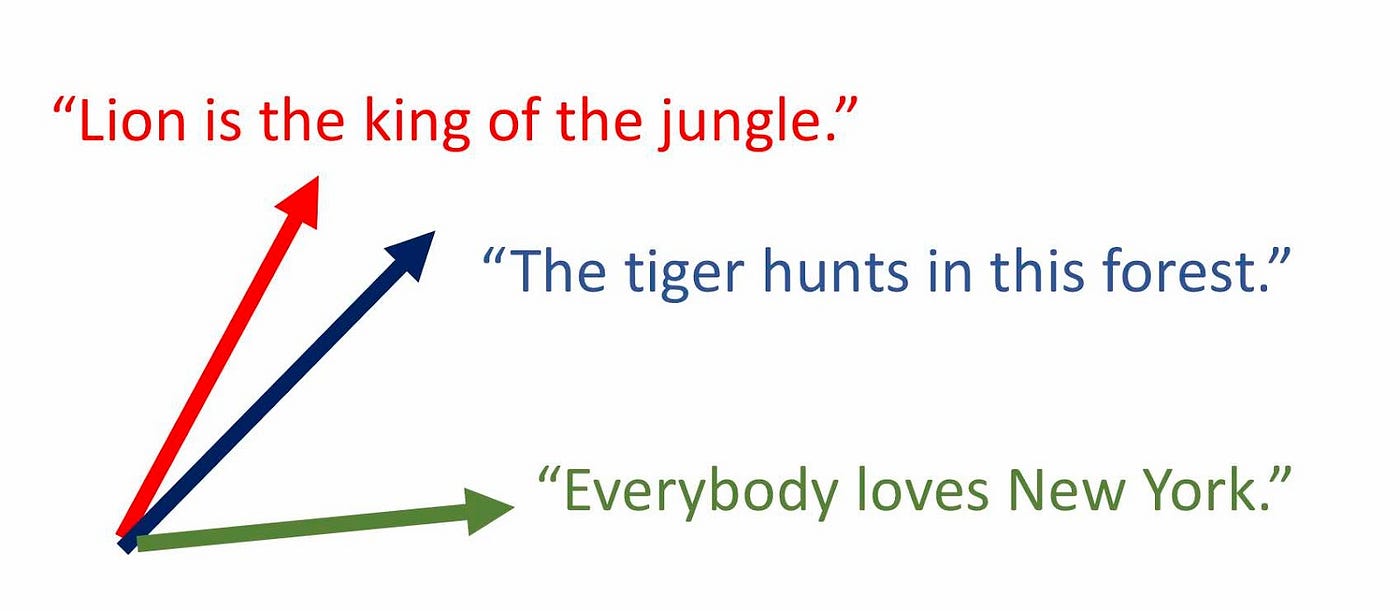
语义嵌入是现代搜索技术背后的主要工作马之一。语义搜索算法不是直接通过词频（例如，BM25）来匹配查询和候选，而是首先将文本 \(x\) 转换为特征向量 \(\phi(x)\)，然后在该向量空间中定义一个距离度量来比较相似性。这些特征向量，被称为“向量嵌入”，通常在大型文本语料库上进行端到端训练，以便编码文本的语义意义。例如，同义词被嵌入到向量空间的相似区域，词语之间的关系通常通过代数运算揭示（参见图 1 的示例）。由于这些原因，文本的向量嵌入也被称为语义嵌入。有了查询和搜索候选文档的语义嵌入，搜索算法通常可以简化为找到最相似的向量。这种新的搜索方法被称为语义搜索。

与经典信息检索方法（例如，词袋或 TF/IDF）相比，使用语义嵌入解决搜索问题有三个主要优势。首先，它根据文本的意义而不是相似的词语用法返回相关的候选。这有助于发现用非常不同方式描述的同义文本和相似概念。其次，语义搜索通常计算效率更高。候选的向量嵌入可以预先计算并存储在数据结构中。诸如局部敏感哈希 (LSH) 和最大内积搜索 (MIPS) 之类的高度可扩展的草图技术可用于有效地在嵌入空间中查找相似向量。最后但同样重要的是，语义嵌入方法使我们能够直接将相同的搜索算法推广到文本之外，例如多模态搜索。例如，我们能否使用文本查询来搜索没有文本注释的图像？我们能否使用图像查询来搜索网站？通过语义搜索，人们可以简单地使用这些多模态对象最合适的向量嵌入，并使用包含文本和图像的数据集共同训练嵌入。

本教程为您提供了一个轻松入门点，将 AutoMM 部署到语义搜索。

%%capture
!pip3 install ir_datasets
import ir_datasets
import pandas as pd
pd.set_option('display.max_colwidth', None)

2. 数据集¶

在本教程中，我们将使用来自 ir_datasets 包的 NF Corpus (Nutrition Facts) 数据集。我们还将查询数据、文档数据及其相关性数据转换为数据帧。

%%capture
dataset = ir_datasets.load("beir/nfcorpus/test")

# prepare dataset
doc_data = pd.DataFrame(dataset.docs_iter())
query_data = pd.DataFrame(dataset.queries_iter())
labeled_data = pd.DataFrame(dataset.qrels_iter())
label_col = "relevance"
query_id_col = "query_id"
doc_id_col = "doc_id"
text_col = "text"
id_mappings={query_id_col: query_data.set_index(query_id_col)[text_col], doc_id_col: doc_data.set_index(doc_id_col)[text_col]}

标记数据包含查询 ID、文档 ID 及其相关性分数。

labeled_data.head()

	query_id	doc_id	relevance
0	PLAIN-2	MED-2427	2
1	PLAIN-2	MED-10	2
2	PLAIN-2	MED-2429	2
3	PLAIN-2	MED-2430	2
4	PLAIN-2	MED-2431	2

查询数据存储查询 ID 及其相应的查询内容。

query_data.head()

	query_id	text	url
0	PLAIN-2	Do Cholesterol Statin Drugs Cause Breast Cancer?	http://nutritionfacts.org/2015/07/16/do-cholesterol-statin-drugs-cause-breast-cancer/
1	PLAIN-12	Exploiting Autophagy to Live Longer	http://nutritionfacts.org/2015/06/11/exploiting-autophagy-to-live-longer/
2	PLAIN-23	How to Reduce Exposure to Alkylphenols Through Your Diet	http://nutritionfacts.org/2015/04/28/how-to-reduce-exposure-to-alkylphenols-through-your-diet/
3	PLAIN-33	What’s Driving America’s Obesity Problem?	http://nutritionfacts.org/2015/03/24/whats-driving-americas-obesity-problem/
4	PLAIN-44	Who Should be Careful About Curcumin?	http://nutritionfacts.org/2015/02/12/who-should-be-careful-about-curcumin/

我们需要删除搜索中未使用的 URL。

query_data = query_data.drop("url", axis=1)
query_data.head()

	query_id	text
0	PLAIN-2	Do Cholesterol Statin Drugs Cause Breast Cancer?
1	PLAIN-12	Exploiting Autophagy to Live Longer
2	PLAIN-23	How to Reduce Exposure to Alkylphenols Through Your Diet
3	PLAIN-33	What’s Driving America’s Obesity Problem?
4	PLAIN-44	Who Should be Careful About Curcumin?

文档数据包含文档 ID 以及相应的内容。

doc_data.head(1)

	doc_id	text	title	url
0	MED-10	Recent studies have suggested that statins, an established drug group in the prevention of cardiovascular mortality, could delay or prevent breast cancer recurrence but the effect on disease-specific mortality remains unclear. We evaluated risk of breast cancer death among statin users in a population-based cohort of breast cancer patients. The study cohort included all newly diagnosed breast cancer patients in Finland during 1995–2003 (31,236 cases), identified from the Finnish Cancer Registry. Information on statin use before and after the diagnosis was obtained from a national prescription database. We used the Cox proportional hazards regression method to estimate mortality among statin users with statin use as time-dependent variable. A total of 4,151 participants had used statins. During the median follow-up of 3.25 years after the diagnosis (range 0.08–9.0 years) 6,011 participants died, of which 3,619 (60.2%) was due to breast cancer. After adjustment for age, tumor characteristics, and treatment selection, both post-diagnostic and pre-diagnostic statin use were associated with lowered risk of breast cancer death (HR 0.46, 95% CI 0.38–0.55 and HR 0.54, 95% CI 0.44–0.67, respectively). The risk decrease by post-diagnostic statin use was likely affected by healthy adherer bias; that is, the greater likelihood of dying cancer patients to discontinue statin use as the association was not clearly dose-dependent and observed already at low-dose/short-term use. The dose- and time-dependence of the survival benefit among pre-diagnostic statin users suggests a possible causal effect that should be evaluated further in a clinical trial testing statins’ effect on survival in breast cancer patients.	Statin Use and Breast Cancer Survival: A Nationwide Cohort Study from Finland	http://www.ncbi.nlm.nih.gov/pubmed/25329299

与查询数据类似，我们删除 URL 列。我们还需要将所有有效文本连接到一个列中。

doc_data[text_col] = doc_data[[text_col, "title"]].apply(" ".join, axis=1)
doc_data = doc_data.drop(["title", "url"], axis=1)
doc_data.head(1)

	doc_id	text
0	MED-10	Recent studies have suggested that statins, an established drug group in the prevention of cardiovascular mortality, could delay or prevent breast cancer recurrence but the effect on disease-specific mortality remains unclear. We evaluated risk of breast cancer death among statin users in a population-based cohort of breast cancer patients. The study cohort included all newly diagnosed breast cancer patients in Finland during 1995–2003 (31,236 cases), identified from the Finnish Cancer Registry. Information on statin use before and after the diagnosis was obtained from a national prescription database. We used the Cox proportional hazards regression method to estimate mortality among statin users with statin use as time-dependent variable. A total of 4,151 participants had used statins. During the median follow-up of 3.25 years after the diagnosis (range 0.08–9.0 years) 6,011 participants died, of which 3,619 (60.2%) was due to breast cancer. After adjustment for age, tumor characteristics, and treatment selection, both post-diagnostic and pre-diagnostic statin use were associated with lowered risk of breast cancer death (HR 0.46, 95% CI 0.38–0.55 and HR 0.54, 95% CI 0.44–0.67, respectively). The risk decrease by post-diagnostic statin use was likely affected by healthy adherer bias; that is, the greater likelihood of dying cancer patients to discontinue statin use as the association was not clearly dose-dependent and observed already at low-dose/short-term use. The dose- and time-dependence of the survival benefit among pre-diagnostic statin users suggests a possible causal effect that should be evaluated further in a clinical trial testing statins’ effect on survival in breast cancer patients. Statin Use and Breast Cancer Survival: A Nationwide Cohort Study from Finland

数据集中有 323 个查询，3633 个文档和 12334 个相关性分数。

3. `NDCG` 评估¶

用户最关注第一个结果，然后是第二个，依此类推。因此，精确率对于排名靠前的结果最为重要。在本教程中，我们使用归一化折损累积增益 (NDCG) 来衡量排名性能。

3.1 CG、DCG、IDCG 和 NDCG 公式¶

为了理解 NDCG 指标，我们必须首先理解 CG（累积增益）和 DCG（折损累积增益），以及理解我们在使用 DCG 及其相关度量时所做的两个假设：

高度相关的文档在搜索引擎结果列表中的位置越靠前越有用。
高度相关的文档比边缘相关的文档更有用，边缘相关的文档比不相关的文档更有用

首先，原始的累积增益 (CG)，它累加到指定排名位置 \(p\) 的相关性分数 (\(rel\))

\[ \mathrm{CG}_p = \sum_{i=1}^p \mathrm{rel}_i. \]

然后，折损累积增益 (DCG)，它根据结果中每个相关性分数的位置进行对数惩罚

\[ \mathrm{DCG}_p = \sum_{i=1}^p \frac{\mathrm{rel}_i}{\log_2(i + 1)}. \]

接下来，理想 DCG (IDCG)，它是基于给定评分的最佳可能结果的 DCG

\[ \mathrm{IDCG}_p = \sum_{i=1}^{|\mathrm{REL}_p|} \frac{\mathrm{rel}_i}{\log_2(i + 1)}. \]

其中 \(|mathrm{REL}_p|\) 是语料库中直到位置 \(p\) 的相关文档列表（按相关性排序）。

最后是 NDCG

\[ \mathrm{NDCG}_p = \frac{\mathrm{DCG}_p}{\mathrm{IDCG}_p}. \]

我们提供了一个实用函数来计算排名分数。此外，我们还支持在不同截止值下衡量 NDCG。

from autogluon.multimodal.utils import compute_ranking_score
cutoffs = [5, 10, 20]

---------------------------------------------------------------------------
ImportError                               Traceback (most recent call last)
Cell In[9], line 1
----> 1 from autogluon.multimodal.utils import compute_ranking_score
      2 cutoffs = [5, 10, 20]

ImportError: cannot import name 'compute_ranking_score' from 'autogluon.multimodal.utils' (/home/ci/autogluon/multimodal/src/autogluon/multimodal/utils/__init__.py)

4. 使用 BM25¶

BM25（或 Okapi BM25）是一种流行的排名算法，目前被 OpenSearch 用于对文档与查询的相关性进行评分。我们将使用 BM25 的 NDCG 分数作为本教程的基线。

4.1 定义公式¶

\[ score_{BM25} = \sum_i^n \mathrm{IDF}(q_i) \frac{f(q_i, D) \cdot (k1 + 1)}{f(q_i, D) + k1 \cdot (1 - b + b \cdot \frac{fieldLen}{avgFieldLen})}\]

其中 \(\mathrm{IDF}(q_i)\) 是第 \(i^{th}\) 个查询项的逆文档频率，BM25 用于此部分的实际公式是

\[ \log(1 + \frac{docCount - f(q_i) + 0.5)}{f(q_i) + 0.5}). \]

\(k1\) 是一个可调的超参数，限制了单个查询项对给定文档分数的影响程度。在 ElasticSearch 中，它默认为 1.2。

\(b\) 是另一个超参数变量，它决定了文档长度与语料库中平均文档长度相比的影响。在 ElasticSearch 中，它默认为 0.75。

在本教程中，我们将使用 rank_bm25 包来避免从头实现算法的复杂性。

4.2 定义函数¶

%%capture
!pip3 install rank_bm25
from collections import defaultdict
import string
import nltk
import numpy as np
from nltk.corpus import stopwords
from nltk.tokenize import word_tokenize
from rank_bm25 import BM25Okapi

nltk.download('stopwords')
nltk.download('punkt')

def tokenize_corpus(corpus):
    stop_words = set(stopwords.words("english") + list(string.punctuation))
    
    tokenized_docs = []
    for doc in corpus:
        tokens = nltk.word_tokenize(doc.lower())
        tokenized_doc = [w for w in tokens if w not in stop_words and len(w) > 2]
        tokenized_docs.append(tokenized_doc)
    return tokenized_docs

def rank_documents_bm25(queries_text, queries_id, docs_id, top_k, bm25):
    tokenized_queries = tokenize_corpus(queries_text)
    
    results = {qid: {} for qid in queries_id}
    for query_idx, query in enumerate(tokenized_queries):
        scores = bm25.get_scores(query)
        scores_top_k_idx = np.argsort(scores)[::-1][:top_k]
        for doc_idx in scores_top_k_idx:
            results[queries_id[query_idx]][docs_id[doc_idx]] = float(scores[doc_idx])
    return results

def get_qrels(dataset):
    """
    Get the ground truth of relevance score for all queries
    """
    qrel_dict = defaultdict(dict)
    for qrel in dataset.qrels_iter():
        qrel_dict[qrel.query_id][qrel.doc_id] = qrel.relevance
    return qrel_dict

def evaluate_bm25(doc_data, query_data, qrel_dict, cutoffs):
    
    tokenized_corpus = tokenize_corpus(doc_data[text_col].tolist())
    bm25_model = BM25Okapi(tokenized_corpus, k1=1.2, b=0.75)
    
    results = rank_documents_bm25(query_data[text_col].tolist(), query_data[query_id_col].tolist(), doc_data[doc_id_col].tolist(), max(cutoffs), bm25_model)
    ndcg = compute_ranking_score(results=results, qrel_dict=qrel_dict, metrics=["ndcg"], cutoffs=cutoffs)
    
    return ndcg

qrel_dict = get_qrels(dataset)
evaluate_bm25(doc_data, query_data, qrel_dict, cutoffs)

5. 使用 AutoMM¶

AutoMM 提供易于使用的 API，用于评估排名性能、提取嵌入和进行语义搜索。

5.1 初始化预测器¶

对于文本数据，我们可以使用问题类型 text_similarity 初始化 MultiModalPredictor。我们需要使用 labeled_data 数据帧中的相应列名指定 query、response 和 label。

%%capture
from autogluon.multimodal import MultiModalPredictor

predictor = MultiModalPredictor(
        query=query_id_col,
        response=doc_id_col,
        label=label_col,
        problem_type="text_similarity",
        hyperparameters={"model.hf_text.checkpoint_name": "sentence-transformers/all-MiniLM-L6-v2"}
    )

5.2 评估排名¶

使用 evaluate API 很容易评估排名性能。在评估期间，预测器自动提取嵌入、计算余弦相似度、对结果进行排名并计算分数。

predictor.evaluate(
        labeled_data,
        query_data=query_data[[query_id_col]],
        response_data=doc_data[[doc_id_col]],
        id_mappings=id_mappings,
        cutoffs=cutoffs,
        metrics=["ndcg"],
    )

我们可以发现相比 BM25 的性能有显著改进。

5.3 语义搜索¶

我们还提供了一个用于语义搜索的实用函数。

from autogluon.multimodal.utils import semantic_search
hits = semantic_search(
        matcher=predictor,
        query_data=query_data[text_col].tolist(),
        response_data=doc_data[text_col].tolist(),
        query_chunk_size=len(query_data),
        top_k=max(cutoffs),
    )

我们根据查询和文档嵌入之间的余弦相似度对文档进行排名。为简单起见，我们使用 torch.topk 并采用线性复杂度 (O(n+k)) 来获取与查询嵌入最相似的 k 个向量嵌入。然而，在实践中，通常使用更高效的相似度搜索方法，例如 Faiss。

5.4 提取嵌入¶

提取嵌入对于将模型部署到工业搜索引擎非常重要。一般来说，系统会离线提取数据库项目的嵌入。在在线搜索期间，只需编码查询数据，然后高效地将查询嵌入与保存的数据库嵌入进行匹配。

query_embeds = predictor.extract_embedding(query_data[[query_id_col]], id_mappings=id_mappings, as_tensor=True)
doc_embeds = predictor.extract_embedding(doc_data[[doc_id_col]], id_mappings=id_mappings, as_tensor=True)

6. 混合 BM25¶

我们正在提出一种新的搜索排名方法，称为混合 BM25，它结合了 BM25 和语义嵌入进行评分。其核心思想是使用 BM25 作为第一阶段检索方法（例如，每个查询召回 1000 个文档），然后使用预训练语言模型（PLM）对所有召回的文档（1000 个文档）进行评分。

然后我们使用如下计算的分数对检索到的文档进行重新排名

\[ score = \beta * normalized\_BM25 + ( 1 - \beta) * score\_of\_plm \]

其中

\[ normalized\_BM25(q_i, D_j) = \frac{\textsf{BM25}(q_i,D_j) - \min_{a\in \mathcal{Q},b\in\mathcal{D}}(\textsf{BM25}(a,b))}{\max_{a\in \mathcal{Q},b\in\mathcal{D}}(\textsf{BM25}(a,b)) - \min_{a\in \mathcal{Q},b\in\mathcal{D}}(\textsf{BM25}(a,b))},\]

而 \(\beta\) 是一个可调参数，在本教程中我们将其\(0.3\)设为默认值。

6.1 定义函数¶

import torch
from autogluon.multimodal.utils import compute_semantic_similarity

def hybridBM25(query_data, query_embeds, doc_data, doc_embeds, recall_num, top_k, beta):
    # Recall documents with BM25 scores
    tokenized_corpus = tokenize_corpus(doc_data[text_col].tolist())
    bm25_model = BM25Okapi(tokenized_corpus, k1=1.2, b=0.75)
    bm25_scores = rank_documents_bm25(query_data[text_col].tolist(), query_data[query_id_col].tolist(), doc_data[doc_id_col].tolist(), recall_num, bm25_model)
    
    all_bm25_scores = [score for scores in bm25_scores.values() for score in scores.values()]
    max_bm25_score = max(all_bm25_scores)
    min_bm25_score = min(all_bm25_scores)

    q_embeddings = {qid: embed for qid, embed in zip(query_data[query_id_col].tolist(), query_embeds)}
    d_embeddings = {did: embed for did, embed in zip(doc_data[doc_id_col].tolist(), doc_embeds)}
    
    query_ids = query_data[query_id_col].tolist()
    results = {qid: {} for qid in query_ids}
    for idx, qid in enumerate(query_ids):
        rec_docs = bm25_scores[qid]
        rec_doc_emb = [d_embeddings[doc_id] for doc_id in rec_docs.keys()]
        rec_doc_id = [doc_id for doc_id in rec_docs.keys()]
        rec_doc_emb = torch.stack(rec_doc_emb)
        scores = compute_semantic_similarity(q_embeddings[qid], rec_doc_emb)
        scores[torch.isnan(scores)] = -1
        top_k_values, top_k_idxs = torch.topk(
            scores,
            min(top_k + 1, len(scores[0])),
            dim=1,
            largest=True,
            sorted=False,
        )

        for doc_idx, score in zip(top_k_idxs[0], top_k_values[0]):
            doc_id = rec_doc_id[int(doc_idx)]
            # Hybrid scores from BM25 and cosine similarity of embeddings
            results[qid][doc_id] = \
                (1 - beta) * float(score.numpy()) \
                + beta * (bm25_scores[qid][doc_id] - min_bm25_score) / (max_bm25_score - min_bm25_score)
    
    return results


def evaluate_hybridBM25(query_data, query_embeds, doc_data, doc_embeds, recall_num, beta, cutoffs):
    results = hybridBM25(query_data, query_embeds, doc_data, doc_embeds, recall_num, max(cutoffs), beta)
    ndcg = compute_ranking_score(results=results, qrel_dict=qrel_dict, metrics=["ndcg"], cutoffs=cutoffs)
    return ndcg

recall_num = 1000
beta = 0.3
query_embeds = predictor.extract_embedding(query_data[[query_id_col]], id_mappings=id_mappings, as_tensor=True)
doc_embeds = predictor.extract_embedding(doc_data[[doc_id_col]], id_mappings=id_mappings, as_tensor=True)
evaluate_hybridBM25(query_data, query_embeds, doc_data, doc_embeds, recall_num, beta, cutoffs)

我们成功改进了相较于朴素 BM25 的排名分数。

7. 总结¶

在本教程中，我们展示了如何使用 AutoMM 进行语义搜索，并展示了相较于经典 BM25 的明显改进。我们通过结合 BM25 和 AutoMM（混合 BM25）进一步提高了排名分数。